Performance profiling
Low latency and high throughput performance are critical factors in many DNN applications. For performance optimization, model developers and ML engineers must understand the model performance and be able to analyze bottlenecks. To assist developers with this process, Furiosa SDK provides a profiling tool.
Trace Analysis
Trace analysis provides structured data on execution time by step, by actually executing model inference task. You can also visualize the data using the Trace Event Profiling Tool function of the Chrome web browser.
Though small, trace generation generates temporal overheads as it measures time for each step and writes the results to a file. It is thus not enabled by default. You can create trace by using one of the following methods.
Enabling trace generation through environment variables
You can enable trace generation by setting the path of the file to which the trace result will be written in FURIOSA_PROFILER_OUTPUT_PATH. The advantage of this method is that the code remains unchanged. The downside is that you cannot set a specific section or category for measurement.
cd furiosa-sdk/examples/inferences
export FURIOSA_PROFILER_OUTPUT_PATH=`pwd`/tracing.json
./image_classification.sh ../assets/images/car.jpeg

ls -l ./tracing.json
-rw-r--r--@ 1 furiosa  furiosa  605054 Jun  15 02:02 tracing.json
If you enable trace generation through environment variables as described above, a JSON file will be written to the path specified by the environment variable FURIOSA_PROFILER_OUTPUT_PATH.
If you enter chrome://tracing in Chrome’s address bar, the trace viewer will start. Click the Load button in the upper left corner of the trace viewer, and select the saved file (tracing.json in the example above) to view the trace result.

Enabling trace generation through profiler context
You can also trace a model inference performance by using a Profiler Context in your Python code. The advantages of this method, in comparison to the tracing by environment variable, are as follows:
Allow to enable trace immediately even in interactive environments, such as Python Interpreter or Jupyter Notebook
Allow to specify labels to certain inference runs
Allow to measure specified operator categories selectively
from furiosa.runtime import session, tensor
from furiosa.runtime.profiler import profile

with open("mnist_trace.json", "w") as output:
    with profile(file=output) as profiler:
        with session.create("MNISTnet_uint8_quant_without_softmax.tflite") as sess:
            input_shape = sess.input(0)

            with profiler.record("warm up") as record:
                for _ in range(0, 10):
                    sess.run(tensor.rand(input_shape))

            with profiler.record("trace") as record:
                for _ in range(0, 10):
                    sess.run(tensor.rand(input_shape))
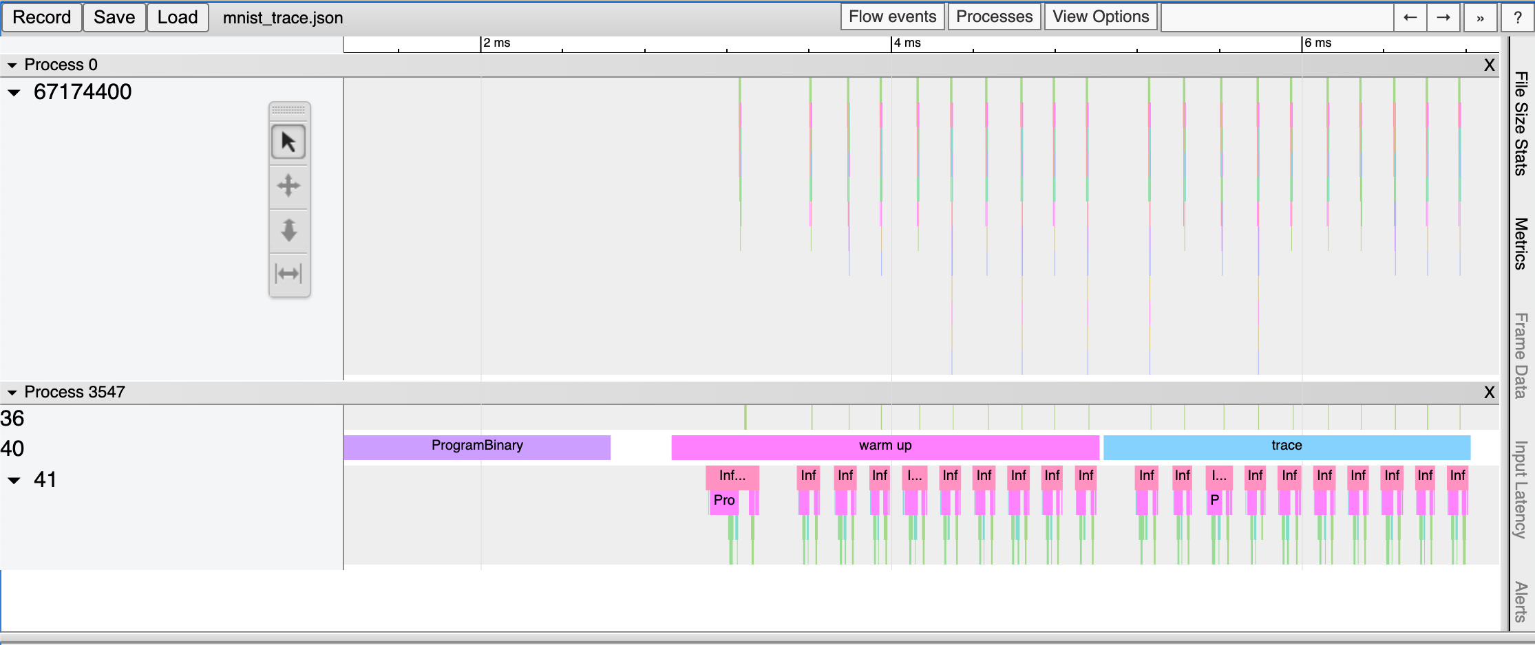
The above is a code example using a profiling context. Once the above Python code is executed, the mnist_trace.json file is created. The trace results are labelled ‘warm up’ and ‘trace’ as shown below.
Trace analysis using Pandas DataFrame
With the measured tracing data, in addition to visualizing it with Chrome Trace Format, it can also be expressed and used in Pandas DataFrame, commonly used for data analysis. These are the advantages in comparison to Chrome Trace Format.
Can be used directly in Python Interpreter or Jupyter Notebook interactive shell
Users can directly access DataFrame for analysis, on top of the reporting function which is provided as default
from furiosa.runtime import session, tensor
from furiosa.runtime.profiler import RecordFormat, profile

with profile(format=RecordFormat.PandasDataFrame) as profiler:
    with session.create("MNISTnet_uint8_quant_without_softmax.tflite") as sess:
        input_shape = sess.input(0)

        with profiler.record("warm up") as record:
            for _ in range(0, 2):
                sess.run(tensor.rand(input_shape))

        with profiler.record("trace") as record:
            for _ in range(0, 2):
                sess.run(tensor.rand(input_shape))

profiler.print_summary() # (1)

profiler.print_inferences() # (2)

profiler.print_npu_executions() # (3)

profiler.print_npu_operators() # (4)

profiler.print_external_operators() # (5)

df = profiler.get_pandas_dataframe() # (6)
print(df[df["name"] == "trace"][["trace_id", "name", "thread.id", "dur"]])
Above is a code example that designates a profiling context format into PandasDataFrame.
When (1) line is executed, the following summary of the results is produced.
================================================
  Inference Results Summary
================================================
Inference counts                : 4
Min latency (ns)                : 258540
Max latency (ns)                : 650018
Mean latency (ns)               : 386095
Median latency (ns)             : 317912
90.0 percentile latency (ns)    : 564572
95.0 percentile latency (ns)    : 607295
97.0 percentile latency (ns)    : 624384
99.0 percentile latency (ns)    : 641473
99.9 percentile latency (ns)    : 649163
When (2) line is executed, duration of one inference query is shown.
                            trace_id           span_id  thread.id     dur
40   daf4d8ed300bc4f93901a978111b44f9  d5ac7df24cfd0408         45  650018
81   02e6fb6504e6f7a1312272077a2ca480  313be2a0fb70dc4f         45  365199
124  713e7a122436acbeeafd1339499a7bed  f4402ab5ea873f46         45  258540
173  7e754c14f342d3eb3f4efbc615d15d8a  4f67a754e72e2211         45  270625
When (3) line is executed, elapsed times of NPU executions will be shown:
                          trace_id           span_id  pe_index  execution_index  NPU Total  NPU Run  NPU IoWait
0  e3917c06e01d136ddb98299da74748d8  1b99d7c6574c1c29         0                0      10902     8559        2343
1  a867049bb2db14e62cebe3dc18546923  f5cd3ba0d885fab4         0                0      10901     8557        2344
2  05bfa81f1579ac8089ac75588f36a747  e7e847b44ce11d28         0                0      10997     8557        2440
3  438df7d9beb7fb8c60daaeffbb2c7e76  d2c20e3d9daf21be         0                0      10900     8555        2345
When (4) line is executed, elapsed times of operators will be shown:
                        average elapsed(ns)  count
name
LowLevelConv2d                   1226.187500     16
LowLevelDepthwiseConv2d           757.333333     12
LowLevelPad                       361.416667     12
LowLevelMask                      116.500000      8
LowLevelExpand                      3.000000      8
LowLevelReshape                     3.000000     68
LowLevelSlice                       3.000000      8
When (5) line is executed, the time data for operators in the CPU is shown as below.
                            trace_id           span_id  thread.id        name  operator_index    dur
2    daf4d8ed300bc4f93901a978111b44f9  704e2c8ece98e29e         45    Quantize               0  42929
3    daf4d8ed300bc4f93901a978111b44f9  4a304c8c46be707a         45       Lower               1  72999
34   daf4d8ed300bc4f93901a978111b44f9  cff0f3268f26423d         45     Unlower               2  31812
36   daf4d8ed300bc4f93901a978111b44f9  b3a90233e6eb90f8         45  Dequantize               3   4895
54   02e6fb6504e6f7a1312272077a2ca480  920c7170893cb202         45    Quantize               0  14085
55   02e6fb6504e6f7a1312272077a2ca480  b2508624adaf01a1         45       Lower               1  32360
75   02e6fb6504e6f7a1312272077a2ca480  ed6fc23c0a7cc81e         45     Unlower               2  15655
78   02e6fb6504e6f7a1312272077a2ca480  e2d61265a1fe0ad6         45  Dequantize               3   6128
96   713e7a122436acbeeafd1339499a7bed  20473c3a26d91593         45    Quantize               0   4400
100  713e7a122436acbeeafd1339499a7bed  f71676c0868f1a34         45       Lower               1  28714
118  713e7a122436acbeeafd1339499a7bed  dff936584542ee83         45     Unlower               2  12675
121  713e7a122436acbeeafd1339499a7bed  9d2eaf76f1a6d156         45  Dequantize               3  12227
138  7e754c14f342d3eb3f4efbc615d15d8a  0df3b383e59e5322         45    Quantize               0   6631
142  7e754c14f342d3eb3f4efbc615d15d8a  c15504b489f56503         45       Lower               1  11694
170  7e754c14f342d3eb3f4efbc615d15d8a  cb8f9199904c6065         45     Unlower               2  17573
171  7e754c14f342d3eb3f4efbc615d15d8a  90c1af4de00eebc2         45  Dequantize               3  16021
With line (6), you can access DataFrame from the code and perform direct analysis.
                            trace_id   name  thread.id     dur
150  ec3dd3d28baf03adc6a1ddd5efe319bc  trace         44  778887