Performance Profiling
Low latency and high throughput performance are critical factors in many DNN applications. For performance optimization, model developers and ML engineers must understand the model performance and be able to analyze bottlenecks. To assist developers with this process, Furiosa SDK provides a profiling tool.
Trace Analysis
Trace analysis provides structured data on execution time by step, by actually executing model inference task. You can also visualize the data using the Trace Event Profiling Tool function of the Chrome web browser.
Though small, trace generation generates temporal overheads as it measures time for each step and writes the results to a file. It is thus not enabled by default. You can create trace by using one of the following methods.
Tracing via Environment Variable
You can enable trace generation by setting the path of the file to which the trace result will be written in FURIOSA_PROFILER_OUTPUT_PATH. The advantage of this method is that the code remains unchanged. The downside is that you cannot set a specific section or category for measurement.
git clone https://github.com/furiosa-ai/furiosa-sdk
cd furiosa-sdk/examples/inferences
export FURIOSA_PROFILER_OUTPUT_PATH=`pwd`/tracing.json
./image_classify.py ../assets/images/car.jpg

ls -l ./tracing.json
-rw-r--r-- 1 furiosa furiosa 456493 Jul 27 17:56 ./tracing.json
If you enable trace generation through environment variables as described above, a JSON file will be written to the path specified by the environment variable FURIOSA_PROFILER_OUTPUT_PATH.
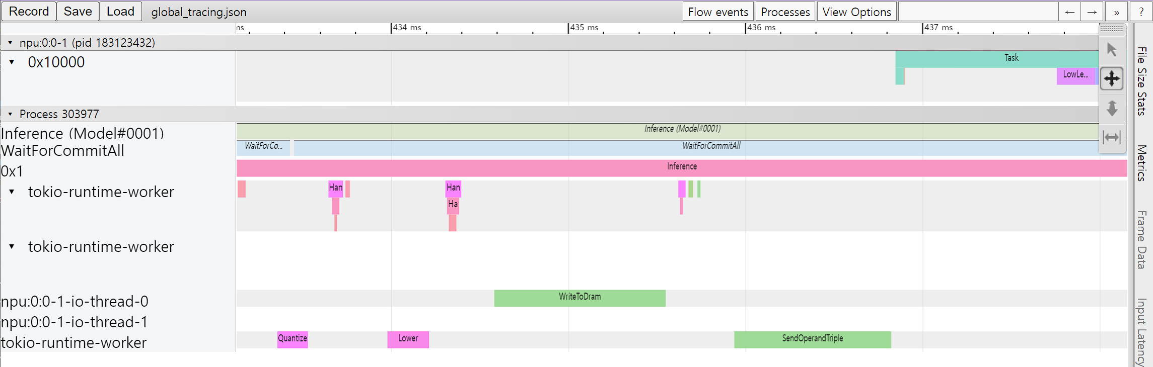
If you enter chrome://tracing in Chrome’s address bar, the trace viewer will start. Click the Load button in the upper left corner of the trace viewer, and select the saved file (tracing.json in the example above) to view the trace result.
Tracing via Profiler Context
You can also trace a model inference performance by using a Profiler Context in your Python code. The advantages of this method, in comparison to the tracing by environment variable, are as follows:
Allow to enable trace immediately even in interactive environments, such as Python Interpreter or Jupyter Notebook
Allow to specify labels to certain inference runs
Allow to measure specified operator categories selectively
#!/usr/bin/env python

import numpy as np
from furiosa.runtime.profiler import profile
from furiosa.runtime.sync import create_runner

# You can find 'examples' directory of the root of furiosa-sdk source tree
model_path = "examples/assets/quantized_models/imagenet_224x224_mobilenet_v1_uint8_quantization-aware-trained_dm_1.0_without_softmax.tflite"

with open("mobilenet_v1_trace.json", "w") as output:
    with profile(file=output) as profiler:
        with create_runner(model_path) as runner:
            input_shape = runner.model.input(0).shape

            with profiler.record("warm up") as record:
                for _ in range(0, 2):
                    runner.run([np.uint8(np.random.rand(*input_shape))])

            with profiler.record("trace") as record:
                for _ in range(0, 2):
                    runner.run([np.uint8(np.random.rand(*input_shape))])
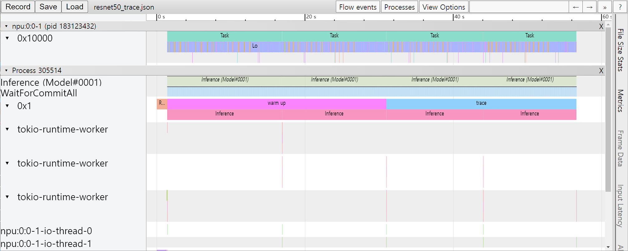
The above is a code example using a profiling context. Once the above Python code is executed, the mnist_trace.json file is created. The trace results are labelled ‘warm up’ and ‘trace’ as shown below.
Pause/Resume of Profiler Context
Tracing long-running jobs can cause following problems:
Produce large trace files which take huge disk space and are difficult to be shared.
Make it hard to identify interesting section when the trace is visualized, without additional processing.
Take much time to produce trace files.
To avoid the above issues, the profiler provides an additional API to temporarily pause or resume a profiler within the context. Users can exclude execution they do not want to profile, thereby reducing profiling overhead and trace file size.
The below is an example of pausing profiler not to trace warm up phase between profile.pause and profile.resume.
#!/usr/bin/env python

import numpy as np
from furiosa.runtime.profiler import RecordFormat, profile
from furiosa.runtime.sync import create_runner

# You can find 'examples' directory of the root of furiosa-sdk source tree
model_path = "examples/assets/quantized_models/imagenet_224x224_mobilenet_v1_uint8_quantization-aware-trained_dm_1.0_without_softmax.tflite"

with profile(format=RecordFormat.PandasDataFrame) as profiler:
    with create_runner(model_path) as runner:
        input_shape = runner.model.input(0).shape

        # pause profiling during warmup
        profiler.pause()

        for _ in range(0, 10):
            with profiler.record("warm up") as record:
                runner.run([np.uint8(np.random.rand(*input_shape))])

        # resume profiling
        profiler.resume()

        with profiler.record("trace") as record:
            runner.run([np.uint8(np.random.rand(*input_shape))])

df = profiler.get_pandas_dataframe()

assert len(df[df["name"] == "trace"]) == 1
assert len(df[df["name"] == "warm up"]) == 0
Trace analysis using Pandas DataFrame
With the measured tracing data, in addition to visualizing it with Chrome Trace Format, it can also be expressed and used in Pandas DataFrame, commonly used for data analysis. These are the advantages in comparison to Chrome Trace Format.
Can be used directly in Python Interpreter or Jupyter Notebook interactive shell
Users can directly access DataFrame for analysis, on top of the reporting function which is provided as default
#!/usr/bin/env python

import numpy as np
from furiosa.runtime.profiler import RecordFormat, profile
from furiosa.runtime.sync import create_runner

# You can find 'examples' directory of the root of furiosa-sdk source tree
model_path = "examples/assets/quantized_models/imagenet_224x224_mobilenet_v1_uint8_quantization-aware-trained_dm_1.0_without_softmax.tflite"

with profile(format=RecordFormat.PandasDataFrame) as profiler:
    with create_runner(model_path) as runner:
        input_shape = runner.model.input(0).shape

        with profiler.record("warm up") as record:
            for _ in range(0, 2):
                runner.run([np.uint8(np.random.rand(*input_shape))])

        with profiler.record("trace") as record:
            for _ in range(0, 2):
                runner.run([np.uint8(np.random.rand(*input_shape))])

profiler.print_summary()  # (1)

profiler.print_inferences()  # (2)

profiler.print_npu_executions()  # (3)

profiler.print_npu_operators()  # (4)

profiler.print_external_operators()  # (5)

df = profiler.get_pandas_dataframe()  # (6)
print(df[df["name"] == "trace"][["trace_id", "name", "thread.id", "dur"]])
Above is a code example that designates a profiling context format into PandasDataFrame.
When (1) line is executed, the following summary of the results is produced.
================================================
  Inference Results Summary
================================================
Inference counts                : 4
Min latency (ns)                : 1584494
Max latency (ns)                : 3027309
Mean latency (ns)               : 2136984
Median latency (ns)             : 1968066
90.0 percentile Latency (ns)    : 2752525
95.0 percentile Latency (ns)    : 2889917
97.0 percentile Latency (ns)    : 2944874
99.0 percentile Latency (ns)    : 2999831
99.9 percentile Latency (ns)    : 3024561
When (2) line is executed, duration of one inference query is shown.
┌──────────────────────────────────┬──────────────────┬───────────┬─────────┐
│ trace_id                         ┆ span_id          ┆ thread.id ┆ dur     │
╞══════════════════════════════════╪══════════════════╪═══════════╪═════════╡
│ 7cf3d3b7439cf4c3fac1a47998783102 ┆ 403ada67f1d8220e ┆ 1         ┆ 3027309 │
│ 16d65f6f8f1db256d0f39953855dea72 ┆ 78b065c19c3675ef ┆ 1         ┆ 2111363 │
│ d0534e3a9f19edadab81954ad28ab44f ┆ 9a7addaf0f28c9fe ┆ 1         ┆ 1824769 │
│ 70512188522f45b87cfe4f545de3cf2c ┆ c75f697f8e72d333 ┆ 1         ┆ 1584494 │
└──────────────────────────────────┴──────────────────┴───────────┴─────────┘
When (3) line is executed, elapsed times of NPU executions will be shown:
┌──────────────────────────────────┬──────────────────┬──────────┬─────────────────┬───────────┬─────────┬──────────────────────┐
│ trace_id                         ┆ span_id          ┆ pe_index ┆ execution_index ┆ NPU Total ┆ NPU Run ┆ NPU IoWait           │
╞══════════════════════════════════╪══════════════════╪══════════╪═════════════════╪═══════════╪═════════╪══════════════════════╡
│ 8f6fce6c0e52b4735cae3379732a0943 ┆ 3e1e4a76523cbf89 ┆ 0        ┆ 0               ┆ 119145    ┆ 108134  ┆ 18446744073709540605 │
│ 195366613b1da9b0350c0a3c2a608f42 ┆ 07dff2e92172fabd ┆ 0        ┆ 0               ┆ 119363    ┆ 108134  ┆ 18446744073709540387 │
│ 3b65b8fa3eabfaf8f815ec9f41fcc7d9 ┆ 639a366a7f932a23 ┆ 0        ┆ 0               ┆ 119157    ┆ 108134  ┆ 18446744073709540593 │
│ e48825df32a07e5559f7f50048c08e1f ┆ ecaab4915bfda725 ┆ 0        ┆ 0               ┆ 119219    ┆ 108134  ┆ 18446744073709540531 │
└──────────────────────────────────┴──────────────────┴──────────┴─────────────────┴───────────┴─────────┴──────────────────────┘
When (4) line is executed, elapsed times of operators will be shown:
┌─────────────────────────┬──────────────────────┬───────┐
│ name                    ┆ average_elapsed (ns) ┆ count │
╞═════════════════════════╪══════════════════════╪═══════╡
│ LowLevelConv2d          ┆ 5327.8               ┆ 60    │
│ LowLevelDepthwiseConv2d ┆ 1412.285714          ┆ 56    │
│ LowLevelPad             ┆ 575.785714           ┆ 56    │
│ LowLevelTranspose       ┆ 250.0                ┆ 4     │
│ LowLevelReshape         ┆ 2.0                  ┆ 240   │
│ LowLevelSlice           ┆ 2.0                  ┆ 12    │
│ LowLevelExpand          ┆ 2.0                  ┆ 16    │
└─────────────────────────┴──────────────────────┴───────┘
When (5) line is executed, the time data for operators in the CPU is shown as below.
┌──────────────────────────────────┬──────────────────┬───────────┬────────────┬────────────────┬────────┐
│ trace_id                         ┆ span_id          ┆ thread.id ┆ name       ┆ operator_index ┆ dur    │
╞══════════════════════════════════╪══════════════════╪═══════════╪════════════╪════════════════╪════════╡
│ e7ab6656cc090a8d05992a9e4683b8b7 ┆ 206a1d6f351ca4b1 ┆ 40        ┆ Quantize   ┆ 0              ┆ 136285 │
│ 03636fd6c7dbc42f0a9dd29a7283d3fc ┆ f636740983e095a6 ┆ 40        ┆ Lower      ┆ 1              ┆ 133350 │
│ c9a0858f7e0885a976f51c6cb57d3e0f ┆ bb6c84f88e453055 ┆ 40        ┆ Unlower    ┆ 2              ┆ 44775  │
│ 8777c67ad9fe597139bbd6970362c2fc ┆ 63bac982c7b98aba ┆ 40        ┆ Dequantize ┆ 3              ┆ 14682  │
│ 98aeba2a25b0525166b6a4065ab01774 ┆ 34ccd560571d733f ┆ 40        ┆ Quantize   ┆ 0              ┆ 45465  │
│ 420525dc13ba9624083e0a276f7ee718 ┆ 9f6d342da5eb86bc ┆ 40        ┆ Lower      ┆ 1              ┆ 152748 │
│ cb67393f6949bbbb396053c1e00931ff ┆ 2d724fa6ab8ca024 ┆ 40        ┆ Unlower    ┆ 2              ┆ 67140  │
│ 00424b4f02039ae0ca98388a964062b0 ┆ a5fb9fbd5bffe6a6 ┆ 40        ┆ Dequantize ┆ 3              ┆ 32388  │
│ d7412c59d360067e8b7a2508a30d1079 ┆ 8e426d778fa95722 ┆ 40        ┆ Quantize   ┆ 0              ┆ 71736  │
│ 6820acf9345c5b373c512f6cd5edcbc7 ┆ 2d787c2df381f010 ┆ 40        ┆ Lower      ┆ 1              ┆ 311310 │
│ 84d24b02a95c63c3e40f7682384749e4 ┆ 1236a974a619ff1a ┆ 40        ┆ Unlower    ┆ 2              ┆ 51930  │
│ 8d25dff1cfd6624509cbf95503e93382 ┆ 673efb3bfb8deac6 ┆ 40        ┆ Dequantize ┆ 3              ┆ 12362  │
│ 4cc60ec1eee7d9f3cdd290d07b303a18 ┆ e7903b0a584d6388 ┆ 40        ┆ Quantize   ┆ 0              ┆ 56736  │
│ c5f04d9fea26e5b52c6ec5e5406775fc ┆ 701118dabd065e6f ┆ 40        ┆ Lower      ┆ 1              ┆ 265447 │
│ c5fdfb9cf454da130148e8e364eeee93 ┆ 5cf3750def19c6e8 ┆ 40        ┆ Unlower    ┆ 2              ┆ 35869  │
│ e1e650d23061140404915f1df36daf9c ┆ ddd76ff19b5cd713 ┆ 40        ┆ Dequantize ┆ 3              ┆ 14688  │
└──────────────────────────────────┴──────────────────┴───────────┴────────────┴────────────────┴────────┘
With line (6), you can access DataFrame from the code and perform direct analysis.
                            trace_id   name  thread.id       dur
487  f3b158734e3684f2e043ed41309c4c2d  trace          1  11204385